Pandas End-to-End Example
The indexing capabilities that come with Pandas are incredibly useful. However,
I find myself forgetting the concepts beyond the basics when I haven’t touched
Pandas in a while. This tutorial serves as my own personal reminder but I hope
others will find it helpful as well.
To motivate this, we we’ll explore a baseball dataset and plot batting averages
for some of the greatest players of all time.
Getting Started
Let’s import the packages that we’ll need to do the analysis and generate some plots
import pandas as pd
import numpy as np
import datetime
from bokeh.plotting import figure, show
from bokeh.models import Range1d
from bokeh.models import PrintfTickFormatter, DatetimeTickFormatter
from bokeh.io import output_notebook
output_notebook()
Load Some Data
First, we’ll download historical data from Sean Lahman’s baseball database and then we make sure that the yearID is recognized as a datetime object.
df = pd.read_csv('Batting.csv')  # Download data from http://seanlahman.com/files/database/lahman-csv_2014-02-14.zip
df['yearID'] = pd.to_datetime(df['yearID'], format='%Y', exact=True)
df.head()| playerID | yearID | stint | teamID | lgID | G | G_batting | AB | R | H | ... | SB | CS | BB | SO | IBB | HBP | SH | SF | GIDP | G_old | |
|---|---|---|---|---|---|---|---|---|---|---|---|---|---|---|---|---|---|---|---|---|---|
| 0 | aardsda01 | 2004-01-01 | 1 | SFN | NL | 11 | 11 | 0 | 0 | 0 | ... | 0 | 0 | 0 | 0 | 0 | 0 | 0 | 0 | 0 | 11 |
| 1 | aardsda01 | 2006-01-01 | 1 | CHN | NL | 45 | 43 | 2 | 0 | 0 | ... | 0 | 0 | 0 | 0 | 0 | 0 | 1 | 0 | 0 | 45 |
| 2 | aardsda01 | 2007-01-01 | 1 | CHA | AL | 25 | 2 | 0 | 0 | 0 | ... | 0 | 0 | 0 | 0 | 0 | 0 | 0 | 0 | 0 | 2 |
| 3 | aardsda01 | 2008-01-01 | 1 | BOS | AL | 47 | 5 | 1 | 0 | 0 | ... | 0 | 0 | 0 | 1 | 0 | 0 | 0 | 0 | 0 | 5 |
| 4 | aardsda01 | 2009-01-01 | 1 | SEA | AL | 73 | 3 | 0 | 0 | 0 | ... | 0 | 0 | 0 | 0 | 0 | 0 | 0 | 0 | 0 | NaN |
5 rows × 24 columns
Basic Indexing
With Pandas, we can perform some basic indexing by choosing all rows where the playerID is mantlmi01 (Mickey Mantle).
df[df['playerID'] == 'mantlmi01']| playerID | yearID | stint | teamID | lgID | G | G_batting | AB | R | H | ... | SB | CS | BB | SO | IBB | HBP | SH | SF | GIDP | G_old | |
|---|---|---|---|---|---|---|---|---|---|---|---|---|---|---|---|---|---|---|---|---|---|
| 53662 | mantlmi01 | 1951-01-01 | 1 | NYA | AL | 96 | 96 | 341 | 61 | 91 | ... | 8 | 7 | 43 | 74 | NaN | 0 | 2 | NaN | 3 | 96 |
| 53663 | mantlmi01 | 1952-01-01 | 1 | NYA | AL | 142 | 142 | 549 | 94 | 171 | ... | 4 | 1 | 75 | 111 | NaN | 0 | 2 | NaN | 5 | 142 |
| 53664 | mantlmi01 | 1953-01-01 | 1 | NYA | AL | 127 | 127 | 461 | 105 | 136 | ... | 8 | 4 | 79 | 90 | NaN | 0 | 0 | NaN | 2 | 127 |
| 53665 | mantlmi01 | 1954-01-01 | 1 | NYA | AL | 146 | 146 | 543 | 129 | 163 | ... | 5 | 2 | 102 | 107 | NaN | 0 | 2 | 4 | 3 | 146 |
| 53666 | mantlmi01 | 1955-01-01 | 1 | NYA | AL | 147 | 147 | 517 | 121 | 158 | ... | 8 | 1 | 113 | 97 | 6 | 3 | 2 | 3 | 4 | 147 |
| 53667 | mantlmi01 | 1956-01-01 | 1 | NYA | AL | 150 | 150 | 533 | 132 | 188 | ... | 10 | 1 | 112 | 99 | 6 | 2 | 1 | 4 | 4 | 150 |
| 53668 | mantlmi01 | 1957-01-01 | 1 | NYA | AL | 144 | 144 | 474 | 121 | 173 | ... | 16 | 3 | 146 | 75 | 23 | 0 | 0 | 3 | 5 | 144 |
| 53669 | mantlmi01 | 1958-01-01 | 1 | NYA | AL | 150 | 150 | 519 | 127 | 158 | ... | 18 | 3 | 129 | 120 | 13 | 2 | 2 | 2 | 11 | 150 |
| 53670 | mantlmi01 | 1959-01-01 | 1 | NYA | AL | 144 | 144 | 541 | 104 | 154 | ... | 21 | 3 | 93 | 126 | 6 | 2 | 1 | 2 | 7 | 144 |
| 53671 | mantlmi01 | 1960-01-01 | 1 | NYA | AL | 153 | 153 | 527 | 119 | 145 | ... | 14 | 3 | 111 | 125 | 6 | 1 | 0 | 5 | 11 | 153 |
| 53672 | mantlmi01 | 1961-01-01 | 1 | NYA | AL | 153 | 153 | 514 | 132 | 163 | ... | 12 | 1 | 126 | 112 | 9 | 0 | 1 | 5 | 2 | 153 |
| 53673 | mantlmi01 | 1962-01-01 | 1 | NYA | AL | 123 | 123 | 377 | 96 | 121 | ... | 9 | 0 | 122 | 78 | 9 | 1 | 0 | 2 | 4 | 123 |
| 53674 | mantlmi01 | 1963-01-01 | 1 | NYA | AL | 65 | 65 | 172 | 40 | 54 | ... | 2 | 1 | 40 | 32 | 4 | 0 | 0 | 1 | 5 | 65 |
| 53675 | mantlmi01 | 1964-01-01 | 1 | NYA | AL | 143 | 143 | 465 | 92 | 141 | ... | 6 | 3 | 99 | 102 | 18 | 0 | 0 | 3 | 9 | 143 |
| 53676 | mantlmi01 | 1965-01-01 | 1 | NYA | AL | 122 | 122 | 361 | 44 | 92 | ... | 4 | 1 | 73 | 76 | 7 | 0 | 0 | 1 | 11 | 122 |
| 53677 | mantlmi01 | 1966-01-01 | 1 | NYA | AL | 108 | 108 | 333 | 40 | 96 | ... | 1 | 1 | 57 | 76 | 5 | 0 | 0 | 3 | 9 | 108 |
| 53678 | mantlmi01 | 1967-01-01 | 1 | NYA | AL | 144 | 144 | 440 | 63 | 108 | ... | 1 | 1 | 107 | 113 | 7 | 1 | 0 | 5 | 9 | 144 |
| 53679 | mantlmi01 | 1968-01-01 | 1 | NYA | AL | 144 | 144 | 435 | 57 | 103 | ... | 6 | 2 | 106 | 97 | 7 | 1 | 1 | 4 | 9 | 144 |
18 rows × 24 columns
Note that df['playerID'] == 'mantlmi01' returns a boolean list (rows with playerID matching mantlmi01 will return true and all others will return false) that can then be used to mask the original dataframe.
Applying Function to a Groupby Object (Aggregating Multiple Columns)
Define a Function
In order to calculate the batting average, for a given player, we need to divide the number of hits (H) by the number of at bats (AB).
As an exercise, let’s start by defining a simple function that can be used after we’ve performed a groupby operation.
def get_batting_avg(group):
    """
    """
    result = 0
    if group['AB'].sum() > 0:
        result = 100.0*(group['H']/group['AB']).mean()

    return result
Groupby Year and Player
Next, we can group the data by yearID and playerID
grouped = df.groupby(['yearID', 'playerID'])Get Annual Batting Averages for Each Player
Then, we apply the get_batting_avg to each group.
batting_avg = grouped.apply(get_batting_avg)
The results look like this (with the batting average in the last column)
batting_avg.head()| yearID | playerID | |
|---|---|---|
| 1871-01-01 00:00:00 | abercda01 | 0.000000 |
| addybo01 | 27.118644 | |
| allisar01 | 29.197080 | |
| allisdo01 | 33.082707 | |
| ansonca01 | 32.500000 |
Get Annual Batting Averages for Mickey Mantle, Roger Maris, and Babe Ruth
To get batting averages for specific players, we’ll have to use Pandas’ .loc function to select for a given player.
player = 'mantlmi01'
idx = pd.IndexSlice
mantle_batting_avg = pd.DataFrame(batting_avg.loc[idx[:], idx[player]], columns=['avg'])
mantle_batting_avg.head()| avg | |
|---|---|
| yearID | |
| 1951-01-01 | 26.686217 |
| 1952-01-01 | 31.147541 |
| 1953-01-01 | 29.501085 |
| 1954-01-01 | 30.018416 |
| 1955-01-01 | 30.560928 |
player = 'ruthba01'
ruth_batting_avg = pd.DataFrame(batting_avg.loc[idx[:], idx[player]], columns=['avg'])
player = 'marisro01'
maris_batting_avg = pd.DataFrame(batting_avg.loc[idx[:], idx[player]], columns=['avg'])
Get Annual Batting Averages for Mickey Mantle, Roger Maris, and Babe Ruth
Alternatively, we can get batting averages for a set of players rather than one-by-one
players = ['mantlmi01', 'ruthba01', 'marisro01']
idx = pd.IndexSlice
legends_batting_avg = pd.DataFrame(batting_avg.loc[idx[:], idx[players]], columns=['avg'])
legends_batting_avg| avg | ||
|---|---|---|
| yearID | playerID | |
| 1914-01-01 | ruthba01 | 20.000000 |
| 1915-01-01 | ruthba01 | 31.521739 |
| 1916-01-01 | ruthba01 | 27.205882 |
| 1917-01-01 | ruthba01 | 32.520325 |
| 1918-01-01 | ruthba01 | 29.968454 |
| 1919-01-01 | ruthba01 | 32.175926 |
| 1920-01-01 | ruthba01 | 37.636761 |
| 1921-01-01 | ruthba01 | 37.777778 |
| 1922-01-01 | ruthba01 | 31.527094 |
| 1923-01-01 | ruthba01 | 39.272031 |
| 1924-01-01 | ruthba01 | 37.807183 |
| 1925-01-01 | ruthba01 | 28.969359 |
| 1926-01-01 | ruthba01 | 37.171717 |
| 1927-01-01 | ruthba01 | 35.555556 |
| 1928-01-01 | ruthba01 | 32.276119 |
| 1929-01-01 | ruthba01 | 34.468938 |
| 1930-01-01 | ruthba01 | 35.907336 |
| 1931-01-01 | ruthba01 | 37.265918 |
| 1932-01-01 | ruthba01 | 34.135667 |
| 1933-01-01 | ruthba01 | 30.065359 |
| 1934-01-01 | ruthba01 | 28.767123 |
| 1935-01-01 | ruthba01 | 18.055556 |
| 1951-01-01 | mantlmi01 | 26.686217 |
| 1952-01-01 | mantlmi01 | 31.147541 |
| 1953-01-01 | mantlmi01 | 29.501085 |
| 1954-01-01 | mantlmi01 | 30.018416 |
| 1955-01-01 | mantlmi01 | 30.560928 |
| 1956-01-01 | mantlmi01 | 35.272045 |
| 1957-01-01 | mantlmi01 | 36.497890 |
| marisro01 | 23.463687 | |
| 1958-01-01 | mantlmi01 | 30.443160 |
| marisro01 | 23.607876 | |
| 1959-01-01 | mantlmi01 | 28.465804 |
| marisro01 | 27.251732 | |
| 1960-01-01 | mantlmi01 | 27.514231 |
| marisro01 | 28.256513 | |
| 1961-01-01 | mantlmi01 | 31.712062 |
| marisro01 | 26.949153 | |
| 1962-01-01 | mantlmi01 | 32.095491 |
| marisro01 | 25.593220 | |
| 1963-01-01 | mantlmi01 | 31.395349 |
| marisro01 | 26.923077 | |
| 1964-01-01 | mantlmi01 | 30.322581 |
| marisro01 | 28.070175 | |
| 1965-01-01 | mantlmi01 | 25.484765 |
| marisro01 | 23.870968 | |
| 1966-01-01 | mantlmi01 | 28.828829 |
| marisro01 | 23.275862 | |
| 1967-01-01 | mantlmi01 | 24.545455 |
| marisro01 | 26.097561 | |
| 1968-01-01 | mantlmi01 | 23.678161 |
| marisro01 | 25.483871 |
Get Aggregated Annual Batting Averages
Finally, we can get annual batting averages for the entire league by taking the mean (np.mean) across batting averages for each year.
In other words, we choose a single year and calculate the average batting average across all players for that year and then repeat this for each year.
all_batting_avg = batting_avg.groupby(level=['yearID']).agg({'avg': np.mean})
all_batting_avg.head()| avg | |
|---|---|
| yearID | |
| 1871-01-01 00:00:00 | 25.431261 |
| 1872-01-01 00:00:00 | 24.555224 |
| 1873-01-01 00:00:00 | 24.974896 |
| 1874-01-01 00:00:00 | 24.023281 |
| 1875-01-01 00:00:00 | 22.016575 |
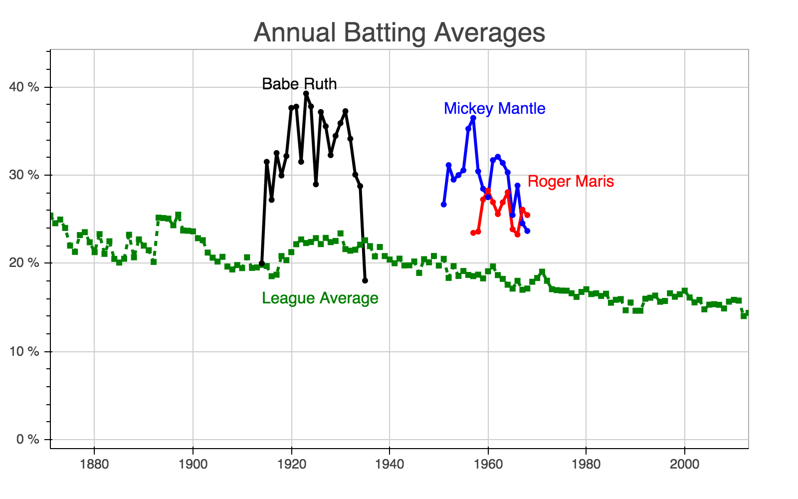
Plot Batting Averages Over Time
Now, we will plot the performance of the legendary players with respect to the league average using Bokeh.
def get_timestamp(time):
    """
    Convert datetime to epoch time for Bokeh
    """

    delta = (pd.to_datetime(time).to_datetime() - datetime.datetime(1970, 1, 1))
    return 1000*delta.total_seconds()
# Get xlim, ylim
minx = min(all_batting_avg.index.values.min(), ruth_batting_avg.index.values.min())
maxx = max(all_batting_avg.index.values.max(), ruth_batting_avg.index.values.max())
miny = min(all_batting_avg.values.min(), ruth_batting_avg.values.min())
maxy = max(all_batting_avg.values.max(), ruth_batting_avg.values.max())
p = figure(width=800, height=500, x_axis_type="datetime")
# Draw lines
p.set(x_range=Range1d(minx, maxx), y_range=Range1d(-1, maxy+5), title='Annual Batting Averages')
p.line(all_batting_avg.index.values, all_batting_avg.values.flatten(), line_width=3, line_color='green', line_join='round', line_dash=[5,5])
p.line(mantle_batting_avg.index.values, mantle_batting_avg.values.flatten(), line_width=3, line_color='blue', line_join='round')
p.line(maris_batting_avg.index.values, maris_batting_avg.values.flatten(), line_width=3, line_color='red', line_join='round')
p.line(ruth_batting_avg.index.values, ruth_batting_avg.values.flatten(), line_width=3, line_color='black', line_join='round')
# Draw shapes
p.square(all_batting_avg.index.values, all_batting_avg.values.flatten(), size=5, line_color='green', fill_color='green')
p.circle(mantle_batting_avg.index.values, mantle_batting_avg.values.flatten(), size=5, line_color='blue', fill_color='blue')
p.circle(maris_batting_avg.index.values, maris_batting_avg.values.flatten(), size=5, line_color='red', fill_color='red')
p.circle(ruth_batting_avg.index.values, ruth_batting_avg.values.flatten(), size=5, line_color='black', fill_color='black')
# Define Axes Format
p.xaxis[0].formatter = DatetimeTickFormatter(formats=dict(years=["%Y"]))
p.yaxis[0].formatter = PrintfTickFormatter(format="%0.0f %%")
# Write text on plot
p.text(get_timestamp(mantle_batting_avg.index.values.min()), mantle_batting_avg.values.max(), text=["Mickey Mantle"], text_color='blue')
p.text(get_timestamp(maris_batting_avg.index.values.max()), maris_batting_avg.values.max(), text=["Roger Maris"], text_color='red')
p.text(get_timestamp(ruth_batting_avg.index.values.min()), ruth_batting_avg.values.max(), text=["Babe Ruth"], text_color='black')
show(p)